Eigenvalues of Sequences, Matrices and ODEs

初中临近毕业，准备高中自招，误打误撞买了本高考自招指南。第一次见到了线性递推数列的特征根解法。后来学习物理竞赛，学解微分方程，在线性常系数常微分方程的解法中了解到了特征根解法。学线代的时候又接触到了矩阵的特征值。在数列、微分方程、矩阵三个不同的领域中都见到了“特征值”这个名字，难道仅仅是因为他们都刻画了问题的特征吗？当时我想，一定不是的。或许这些特征值是同一个特征值。

As I was finishing middle school and preparing for high schools' own entrance exams, I accidentally picked up a prep book for the gaokao and universities' own admissions tests instead. That was where I first encountered the characteristic-root method for linear recurrence sequences. Later, while studying differential equations for physics Olympiads, I met the characteristic-root method again, this time for linear ordinary differential equations with constant coefficients. Then linear algebra brought me matrix eigenvalues. Sequences, differential equations, matrices: three different subjects, all using this name, “eigenvalue.” Was it just because they all characterize something about the problem? I thought it had to be more than that. Perhaps these were actually the same eigenvalues.

因为本人水平较低，这个问题断断续续地想了好几年，逐渐从各个角度撺出了一些头绪。本文对这些想法做一个介绍和总结，试图一窥这些特征值之间的关系。下文中很多内容是常见的数学基础知识，在各种教材中都可以见到，在此一并做一个回顾，故本文只需一点点微积分和线代基础即可阅读；另一些想法和关联是我自己凭空捏造出来的，完全有可能是瞎掰，望读者不吝指正。或许还有一些显而易见、呼之欲出的关联，因本人知识水平有限，无法注意到，望读者提点。

Since I am not particularly good at this, I spent several years thinking about the question on and off, gradually piecing together a few ideas from different directions. This article introduces and collects those ideas, in the hope of getting a glimpse of how these eigenvalues are related. Much of what follows is standard basic mathematics, found in all sorts of textbooks; I review it here too, so you only need a little calculus and linear algebra. Some of the other ideas and connections are things I made up out of thin air and could be complete nonsense. Please do point out any mistakes. There may also be obvious connections staring me in the face that I simply do not know enough to notice. Do enlighten me.

我会先介绍预备知识引入，如果你已经会了的话请放心跳过。然后会探究数列、矩阵和微分方程中的特征值的关系。

I will start with the background. If you already know it, feel free to skip ahead. Then we will explore the relationship between eigenvalues in sequences, matrices, and differential equations.

相信高中学过数列的朋友们都听说过数列的特征根解法，下面我们以二阶齐次线性递推数列的特征根解法为例，做一个简单的介绍。高阶的版本同理。

If you studied sequences in high school, you have probably heard of the characteristic-root method. Here is a brief introduction using a second-order homogeneous linear recurrence. The higher-order case works the same way.

聪明的你或许已经注意到了我放着简单的x不用，偏要用TeX代码好长的\lambda，打得我累死了。以及特征根可以为复数，想一想，复数时会怎样？

You may already have noticed that I passed over the perfectly simple x and insisted on \lambda, with its annoyingly long TeX command. My fingers are exhausted. Also, the characteristic roots can be complex. Have a think: what happens then?

下面我们来做个简单的证明，这一证明常见于各种高考学教材，大家会注意到这一方法基本完全没有intuition指导，乍看起来莫名其妙，非常具有技巧性，让人好奇是怎么拍脑袋想出来的。

Let us give a quick proof, the sort found in all kinds of gaokao-prep books. You will notice that there is basically no intuition guiding it. At first sight it is baffling, full of tricks, and makes you wonder how anyone pulled it out of a hat.

有韦达定理可知 \(p=-\lambda_1-\lambda_2, q=\lambda_1\lambda_2\) ，代入递推式得到

By Vieta’s formulas, \(p=-\lambda_1-\lambda_2, q=\lambda_1\lambda_2\). Substitute into the recurrence to get

\[a_{n+2}-(\lambda_1+\lambda_2)a_{n+1}+\lambda_1\lambda_2a_n=0，\\\]

\[a_{n+2}-(\lambda_1+\lambda_2)a_{n+1}+\lambda_1\lambda_2a_n=0，\\\]

接下来神来之笔地移项，得到

Now, with a stroke of inspiration, rearrange the terms:

\[a_{n+2}-\lambda_1a_{n+1}=\lambda_2(a_{n+1}-\lambda_1a_{n})，\\\]

\[a_{n+2}-\lambda_1a_{n+1}=\lambda_2(a_{n+1}-\lambda_1a_{n})，\\\]

可见莫名其妙得到了一个等比数列，解之，得

Somehow a geometric sequence has appeared out of nowhere. Solve it to get

\[a_{n+1}-\lambda_1a_n=C\lambda_2^{n+1},\\\]

\[a_{n+1}-\lambda_1a_n=C\lambda_2^{n+1},\\\]

然后凑一凑，

Then fiddle with it a little,

\[\frac{a_{n+1}}{\lambda_1^{n+1}}-\frac{a_n}{{\lambda_1^{n}}}=C\frac{\lambda_2^{n+1}}{{\lambda_1^{n+1}}},\\\]

\[\frac{a_{n+1}}{\lambda_1^{n+1}}-\frac{a_n}{{\lambda_1^{n}}}=C\frac{\lambda_2^{n+1}}{{\lambda_1^{n+1}}},\\\]

再累加，这时由于要求右侧等比数列的和，需要对公比是否等于1分类，

and sum. Since we need the sum of the geometric sequence on the right, we have to split into cases according to whether the common ratio is 1.

若 \(\lambda_1=\lambda_2=\lambda\) ，则

If \(\lambda_1=\lambda_2=\lambda\), then

\[\frac{a_n}{{\lambda^{n}}}=C_1n+C_2,\\\]

\[\frac{a_n}{{\lambda^{n}}}=C_1n+C_2,\\\]

若 \(\lambda_1\ne\lambda_2\) ，应用等比数列求和公式可得

If \(\lambda_1\ne\lambda_2\), the geometric-series formula gives

\[\frac{a_n}{{\lambda_1^{n}}}=C_1+C_2\frac{\lambda_2^n}{\lambda_1^n}.{\blacksquare}\\\]

\[\frac{a_n}{{\lambda_1^{n}}}=C_1+C_2\frac{\lambda_2^n}{\lambda_1^n}.{\blacksquare}\\\]

希望你还没有因为枯燥的技巧性证明离开。

I hope you have not left because of this dry, trick-laden proof.

先推荐3b1b的系列视频，学线代杀人越货必备。

First, a recommendation: 3b1b’s video series. Essential kit for your linear-algebra exploits.

下面来简单介绍一下特征值。下列论述中若有不理解请直接到3b1b的视频里找对应章节。

Here is a quick introduction to eigenvalues. If anything below is unclear, go straight to the corresponding episode of 3b1b’s series.

首先，矩阵描述了线性变换，一种理解是对基的变换，即将向量在一组基下的分量表示，变换到另一组基下的分量表示；另一种理解是对向量的变换，即将一个向量变换为另一个向量。

First, matrices describe linear transformations. One way to understand this is as a change of basis: converting the components of a vector in one basis into its components in another. Another is as a transformation of vectors: taking one vector to another.

我们先取后一种理解。

Let us use the second interpretation for now.

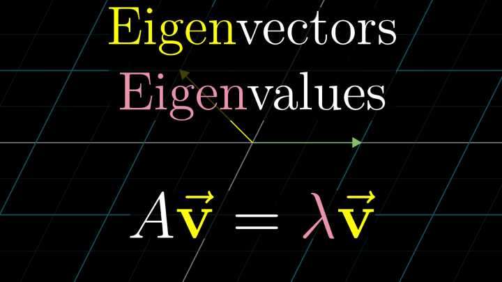
那么对一个线性变换 \(A\) ，可能存在一些向量 \(x\) ，在这个变换下方向不变。用数学的语言，即 \(Ax=\lambda x\) 。我们把这种向量称为 \(A\) 的特征向量，对应的常数 \(\lambda\) 称为对应的特征值。

For a linear transformation \(A\), there may be vectors \(x\) whose direction does not change under the transformation. Mathematically, \(Ax=\lambda x\). We call such vectors eigenvectors of \(A\), and the corresponding constant \(\lambda\) the eigenvalue.

为什么特征值值得我们研究？

Why are eigenvalues worth studying?

依我看，是因为它把矩阵的乘法变成了常数的乘法，在许多场合可以大大简化计算。

To me, it is because they turn matrix multiplication into multiplication by a constant, which can make calculations much simpler.

最基本的求矩阵特征值的方法便是从定义 \(Ax=\lambda x\) 出发，我们做移项，得

The most basic way to find matrix eigenvalues starts from the definition \(Ax=\lambda x\). Rearrange to get

\[(A-\lambda I)x=0,\\\]

\[(A-\lambda I)x=0,\\\]

其中 \(I\) 代表单位矩阵。为了得到非平凡解（ \(x\ne 0\) ），必须要求前面的矩阵的行列式为零：

Here \(I\) is the identity matrix. For a nontrivial solution, \(x\ne 0\), the determinant of the matrix in front must vanish:

\[|A-\lambda I|=0，\\\]

\[|A-\lambda I|=0，\\\]

该方程称为矩阵 \(A\) 的特征方程。

This is called the characteristic equation of the matrix \(A\).

我们举一个例子 \(A=\begin{pmatrix} -p & -q \\ 1 & 0 \end{pmatrix}\) （为什么我们要举这个例子？），

Take the example \(A=\begin{pmatrix} -p & -q \\ 1 & 0 \end{pmatrix}\). Why this example, I wonder?

特征方程就是 \[\begin{vmatrix} -p-\lambda & -q \\ 1 & -\lambda \end{vmatrix}=0,\\\]

Its characteristic equation is \[\begin{vmatrix} -p-\lambda & -q \\ 1 & -\lambda \end{vmatrix}=0,\\\].

展开得到

Expanding gives

\[\lambda^2+p\lambda+q=0.\\\]

\[\lambda^2+p\lambda+q=0.\\\]

上式的两个根即为该矩阵的两个特征值。再代入定义式便可得到对应的特征向量。

The two roots are the matrix’s two eigenvalues. Substitute them back into the defining equation to find the corresponding eigenvectors.

比如方程 \(Ax=0\) 有两个解 \(x_1,x_2,\) 那么他们的线性叠加 \(C_1x_1+C_2x_2\) 也是解。

For example, if \(Ax=0\) has two solutions \(x_1,x_2,\), their linear combination \(C_1x_1+C_2x_2\) is also a solution.

学物理的同学可能经常会遇到线性微分方程，比如单摆的运动方程 \(\ddot{\theta}+\frac{g}{l}\theta=0\) 。

Physics students often run into linear differential equations, such as the equation of motion of a simple pendulum, \(\ddot{\theta}+\frac{g}{l}\theta=0\).

解得时候老师经常会用“猜解”这种说辞糊弄人，我们拿二阶的方程做个例子。高阶同理。

When solving these, instructors often fob us off with “guess a solution.” Let us take a second-order equation as an example. Higher orders work the same way.

\[\ddot{x}+p\dot{x}+qx=0\\\]

\[\ddot{x}+p\dot{x}+qx=0\\\]

（以后我们在函数上打点即表示对时间 \(t\) 的导数，两个点就是二阶导，以此类推。同时我们有时将求导这件事写成一个算符 \(D\) 的形式，比如 \(Dx=\dot{x}\) 。想一下，为什么要写成这种难看的形式？）

(From here on, a dot over a function means differentiation with respect to time \(t\); two dots mean a second derivative, and so on. Sometimes we will also write differentiation as an operator \(D\), for example \(Dx=\dot{x}\). Have a think: why write it in this ugly form?)

猜 \(x=Ce^{\lambda t}\) ，代入方程，由于我们知道 \(De^{\lambda t}=\lambda e^{\lambda t}\) （有没有联想到什么？）,约去指数部分，可得

Guess \(x=Ce^{\lambda t}\) and substitute. Since we know \(De^{\lambda t}=\lambda e^{\lambda t}\)—does that remind you of anything?—we can cancel the exponential part to get

\[\lambda^2+p\lambda+q=0.\\\]

\[\lambda^2+p\lambda+q=0.\\\]

上式称为该微分方程的特征方程。解出来两个根 \(\lambda_1,\lambda_2\in\mathbb{C},\)

This is the differential equation’s characteristic equation. Solving it gives two roots, \(\lambda_1,\lambda_2\in\mathbb{C},\).

如果 \(\lambda_1\ne\lambda_2,\) 那么方程的通解为 \(x=C_1e^{\lambda_1 t}+C_2e^{\lambda_2 t}\) 。（老师说这叫叠加原理）

If \(\lambda_1\ne\lambda_2,\), the general solution is \(x=C_1e^{\lambda_1 t}+C_2e^{\lambda_2 t}\). (The instructor says this is the superposition principle.)

如果 \(\lambda_1=\lambda_2=\lambda,\) 那么方程的通解为 \(x=(C_1+C_2t)e^{\lambda t}\) 。（有没有联想到什么？）

If \(\lambda_1=\lambda_2=\lambda,\), the general solution is \(x=(C_1+C_2t)e^{\lambda t}\). (Does that remind you of anything?)

以上这种“不证自明”的猜解方法又透露出了我们在数列板块中熟悉的莫名其妙。只是这次我打算把证明留到后面。在那里，我们将要引入傅里叶变换及拉普拉斯变换。

This supposedly self-evident way of guessing a solution has the same baffling quality we met with sequences. This time, though, I will leave the proof for later, when we introduce Fourier and Laplace transforms.

相信到目前为止，你或许已经从不同板块中的相似式子里看出了一些端倪。年轻的我当时就是在这种好奇地驱使下开始思考其间的关系。以下我们将要开始对其中的关联做一些探究。

By now you may have noticed something in the similar-looking formulas from these different subjects. That was the curiosity that got my younger self thinking about the connections. Now let us start exploring them.

如果你想要休息一下，现在是个好时候。

If you would like a break, this is a good time.

注意：以下内容是我在某个夜晚灵机一动捏造出来的，有可能是错的。

Note: I made the following up in a flash of inspiration one night. It could be wrong.

让我们先来观察对比一下数列递推方程和微分方程（高阶同理）：

First, compare the recurrence relation and the differential equation. Higher orders work the same way:

\(a_{n+2}+pa_{n+1}+qa_n=0,\\ \ddot{x}+p\dot{x}+qx=0.\)

\(a_{n+2}+pa_{n+1}+qa_n=0,\\ \ddot{x}+p\dot{x}+qx=0.\)

特征方程均为

The characteristic equation in both cases is

\[\lambda^2+p\lambda+q=0\\\]

\[\lambda^2+p\lambda+q=0\\\]

你有没有突然觉得，数列每递推一项，就好像多求了一阶导数？

Does it suddenly look as though advancing the recurrence by one term is like taking one more derivative?

基于这个重要的观察，我们或许可以构造一个函数出来，

With that observation, perhaps we can construct a function

让这个函数每多求一次导，就可以生产出数列的一项。

that produces another term of the sequence each time we differentiate it.

函数有自变量，因此我们还要找一个自变量把数列的项给套出来。

A function has an argument, so we also need a value of that argument at which to extract the sequence terms.

我想到了我们最熟悉的多项式函数，并且想不妨就用 \(0\) 把数列套出来，于是我们构造：

I thought of the familiar polynomial functions, and figured we might as well use \(0\) to extract the sequence. So we construct:

\[x=a_0+a_1t+\frac{a_2}{2!}t^2+\dots+\frac{a_n}{n!}t^n+\dots\\\]

\[x=a_0+a_1t+\frac{a_2}{2!}t^2+\dots+\frac{a_n}{n!}t^n+\dots\\\]

（是不是和泰勒展开很像？）

(Looks rather like a Taylor expansion, doesn’t it?)

这样， \(D^nx(0)=a_n\) ，我们便可以从函数中套出数列了。

Now \(D^nx(0)=a_n\), and we can extract the sequence from the function.

（事后证明，这与组合数学中的母函数思想类似，不过我不会组合数学，母函数这个名字还是从OI同学那听来的，便不多说了。）

(It later turned out that this resembles the idea of a generating function in combinatorics. But I do not know combinatorics; I only heard the name from a friend who competed in informatics Olympiads, so I will leave it there.)

接着我们把这个函数代入数列递推式，得到

Substitute this function into the recurrence relation:

\[D^{n+2}x(0)+pD^{n+1}x(0)+qD^{n}x(0)=0.\\\]

\[D^{n+2}x(0)+pD^{n+1}x(0)+qD^{n}x(0)=0.\\\]

为了让它更接近微分方程，我们不妨给这个函数多做点约束。原先递推方程只要求函数在 \(t=0\) 处满足，我们不妨让它在处处均要满足，来试一试。于是我们得到

To make it look more like a differential equation, let us add a constraint. The recurrence only requires the equation to hold at \(t=0\). Why not try requiring it to hold everywhere? We get

\[D^{n+2}x+pD^{n+1}x+qD^{n}x=0.\\\]

\[D^{n+2}x+pD^{n+1}x+qD^{n}x=0.\\\]

这时，如果我们把函数 \(D^nx\) 看作一个整体，记作 \(x_n\) ，则 \(x_n(0)=a_n\) ，而且

Now regard the function \(D^nx\) as a whole and call it \(x_n\). Then \(x_n(0)=a_n\), and

\[\ddot{x}_n+p\dot{x}_n+qx_n=0.\\\]

\[\ddot{x}_n+p\dot{x}_n+qx_n=0.\\\]

至此，我们成功把数列递推方程转化为了微分方程！！

We have turned the recurrence relation into a differential equation!!

我们取信息量最大（求导次数最少）的方程，即n=0，\(x_0=x\) ：

Take the equation with the most information—the fewest derivatives—that is, n=0, \(x_0=x\):

\[\ddot{x}+p\dot{x}+qx=0.\\\]

\[\ddot{x}+p\dot{x}+qx=0.\\\]

用二-3中已经推导的结论，我们得到 \(x=C_1e^{\lambda_1t}+C_2e^{\lambda_2t}\) 或 \(x=(C_1+C_2t)e^{\lambda t}\) 。

Using the result from II.3 gives \(x=C_1e^{\lambda_1t}+C_2e^{\lambda_2t}\) or \(x=(C_1+C_2t)e^{\lambda t}\).

于是 \(a_n=D^nx(0)=C_1\lambda_1^ne^{\lambda_1t}+C_2\lambda_2^ne^{\lambda_2t}|_{t=0}=C_1\lambda_1^n+C_2\lambda_2^n,\)

Thus \(a_n=D^nx(0)=C_1\lambda_1^ne^{\lambda_1t}+C_2\lambda_2^ne^{\lambda_2t}|_{t=0}=C_1\lambda_1^n+C_2\lambda_2^n,\)

或者 \(a_n=D^nx(0)=C_1\lambda^ne^{\lambda t}+nC_2\lambda^ne^{\lambda t}|_{t=0}=(C_1+C_2n)\lambda^n.\)

or \(a_n=D^nx(0)=C_1\lambda^ne^{\lambda t}+nC_2\lambda^ne^{\lambda t}|_{t=0}=(C_1+C_2n)\lambda^n.\).

注意到这里推导的时候有两件事：

Two things to note in this derivation:

1. 为了保持一致性，额外的系数被吸收进了 \(C_1, C_2\) 两个常数里；
2. 第二种情况中，所有求导出含 \(t\) 的项都会因为 \(t=0\) 而消失，故略去不写，而反复应用乘积的求导法则，便会产生 \(n\) 。

1. To keep the expressions consistent, extra coefficients have been absorbed into the two constants \(C_1, C_2\).
2. In the second case, every term containing \(t\) after differentiation vanishes because \(t=0\), so I have left those terms out. Repeated use of the product rule produces \(n\).

由此，我们发现了数列特征根与微分方程特征根的一致性。

So we have found that the characteristic roots of the sequence and the differential equation agree.

我们发现，竟然之前因为等比数列求和公比等于1的奇葩分类也能通过微分方程复现。

Even that bizarre case split over whether the geometric-series ratio is 1 turns up again through the differential equation.

再次重申，上述过程是我拍脑袋想出来的，不保证正确性。

Once again: I dreamed this up myself. No guarantee that it is correct.

这一步的联系是我在学习量子力学的时候学到的，让我们一步一步地来。

I learned this connection while studying quantum mechanics. Let us take it step by step.

首先，想要用线性代数的工具研究函数，我们就必须证明：

First, if we want to study functions using linear algebra, we must show that

我在初学时对这句话感到非常惊艳。

This statement really blew me away when I first learned it.

我们先来回顾一下向量与线性空间的定义。

Let us review the definitions of a vector and a linear space.

以下抄百度百科：

The following is copied from Baidu Baike:

接下来，如果我们定义函数之间的加法为自变量取值对应函数值直接相加，

Now define addition of functions by simply adding their values at each argument.

比如 \(f(x)=x, g(x)=x^2,\) 那么 \(\alpha f(x)+\beta g(x)=\beta x^2+\alpha x\) ，显然后者也是函数。

For example, if \(f(x)=x, g(x)=x^2,\), then \(\alpha f(x)+\beta g(x)=\beta x^2+\alpha x\), which is clearly also a function.

如此可以证明，函数空间也是一个线性空间，而每个函数就是一个向量。

In this way we can show that a function space is a linear space, and each function is a vector.

接下来，我们便可以将平时在线代中发展出的工具应用到函数中。

We can now apply our familiar tools from linear algebra to functions.

比如，我们可以定义内积。

For example, we can define an inner product.

接下来我们引入一组量子力学中的记号，狄拉克记号：

Next, let us introduce some notation from quantum mechanics: Dirac notation.

在线性代数中我们知道，一个向量本身，跟我们所选取的、用来描述他的基底无关。但我们描述它的时候，一般需要选取一组基底，用在各个基底上的分量来表述他。

From linear algebra, we know that a vector itself is independent of the basis we choose to describe it. But to describe it, we usually choose a basis and specify its components in that basis.

下面我们来考察如何把函数这个向量写成分量形式。

Let us see how to write a function, viewed as a vector, in component form.

回忆我们定义函数加法的时候，是要求每个自变量对应的函数值直接相加的。而向量相加，也是各个基底对应的分量直接相加的。从这一点出发，我们希望每个自变量的取值都对应一个基底，而这个对应的函数值则作为这个基底上的分量。

Recall that we defined addition of functions by adding their values at each argument. Vector addition also adds the corresponding components in a basis. This suggests that each possible argument should correspond to a basis vector, with the function value at that argument as its component.

于是我们把整个定义域分割成 \(n\) 个小段，每一段上定义一个基底

Divide the entire domain into \(n\) small intervals, and define a basis vector on each:

\[|x_i\rangle=(0, 0, \dots, 0, 1,0, \dots, 0)^T\\\] ，其中 \(1\) 位于第 \(i\) 项。然后很自然地，我们的函数在这些基上的分量形式就可以定义为

\[|x_i\rangle=(0, 0, \dots, 0, 1,0, \dots, 0)^T\\\], where \(1\) sits in the \(i\)th position. Naturally, we can then define the components of our function in this basis as

\[|f\rangle=(f(x_1), f(x_2), \dots, f(x_n))^T\\\] ，而且有 \(|f\rangle=\sum_{i=1}^nf(x_i)|x_i\rangle\) 。

\[|f\rangle=(f(x_1), f(x_2), \dots, f(x_n))^T\\\], with \(|f\rangle=\sum_{i=1}^nf(x_i)|x_i\rangle\).

当分隔数 \(n\to+\infty\) 时，我们定义的 \(|f\rangle\) 向量便与原来的函数完全一致了。

As the number of subdivisions \(n\to+\infty\), our vector \(|f\rangle\) becomes exactly the original function.

而这个时候，我们所定义的 \(|x_0\rangle\) 就会变成在 \(x_0\) 处为 \(1\) ，其余处处为 \(0\) ，这样的函数我们称作 \(\delta\) 函数： \[|x_0\rangle=\delta(x-x_0)=\begin{cases} 0&x\ne x_0\\ 1& x=x_0. \end{cases}\\\]

Meanwhile, the \(|x_0\rangle\) we defined becomes \(1\) at \(x_0\) and \(0\) everywhere else. We call such a function a \(\delta\) function: \[|x_0\rangle=\delta(x-x_0)=\begin{cases} 0&x\ne x_0\\ 1& x=x_0. \end{cases}\\\].

至此有两个重要的启示：

Two important things to take away:

1. 函数是无穷维的向量。
2. 所谓的 \(f(x)\) ，其实是函数向量 \(|f\rangle\) 在基底 \(|x\rangle\) 上的分量/投影：

1. Functions are infinite-dimensional vectors.
2. What we call \(f(x)\) is actually the component, or projection, of the function vector \(|f\rangle\) onto the basis vector \(|x\rangle\):

(回忆在线性代数中我们可以通过把向量与基底做内积的方法得到对应的分量)

(Recall that in linear algebra, taking the inner product of a vector with a basis vector gives the corresponding component.)

\[f(x)=\int_{-\infty}^{+\infty}\delta(t-x)f(t)dt=\langle x|f\rangle.\\\]

\[f(x)=\int_{-\infty}^{+\infty}\delta(t-x)f(t)dt=\langle x|f\rangle.\\\]

上述是直观的解释，我们还需要证明一下 \(|x_i\rangle\) 这组基的正交性、完备性，我就不证了。

That is the intuitive explanation. We still need to prove that the basis \(|x_i\rangle\) is orthogonal and complete. I will not prove it here.

现在，函数的内积被定义为上面那个鬼样子的原因就一目了然了。

Now it is obvious why the inner product of functions was defined in that strange-looking way.

我们知道普通向量的内积是对应分量直接相乘然后相加，而这里函数内积

For ordinary vectors, an inner product means multiplying corresponding components and adding them up. Our inner product of functions,

\[\langle f|g\rangle=\int_{-\infty}^{+\infty}f^*(x)g(x)dx\\\]

\[\langle f|g\rangle=\int_{-\infty}^{+\infty}f^*(x)g(x)dx\\\]

确实也是对应分量直接相乘然后相加。

does exactly that: multiply corresponding components and add them up.

接下来我们试着把函数的求导运算也放入线性代数的框架下研究。

Next, let us try bringing differentiation into the framework of linear algebra too.

我们知道，在线性代数中，任何一个线性算符，都能用矩阵的形式表达。

We know from linear algebra that any linear operator can be written as a matrix.

而求导运算显然也是线性的，那导数算符是否也有矩阵形式呢？是否也有特征值和特征向量呢？

Differentiation is clearly linear too. Does the derivative operator have a matrix representation? Does it have eigenvalues and eigenvectors?

第一个问题与本文关系不大，大家可以翻Shankar。（其实我这里本来打了一大段，但是敲公式太累了，通通删了。）

The first question is not especially relevant here; you can look it up in Shankar. (I actually wrote a whole long section here, but typing the formulas was too exhausting, so I deleted the lot.)

我们来看第二个问题，要求矩阵的特征值和特征向量，就是解方程

For the second question, finding a matrix’s eigenvalues and eigenvectors means solving

\[Df=\lambda f\\\]

\[Df=\lambda f\\\]

我们把它改写成微分方程 \(\frac{df}{dx}=\lambda f\) 的话，解就显而易见了。

Rewrite this as the differential equation \(\frac{df}{dx}=\lambda f\), and the solution is obvious.

没错，导数算符的特征向量就对应指数函数 \(f(x)=e^{\lambda x}\) 。

That is right: the derivative operator’s eigenvectors correspond to exponential functions \(f(x)=e^{\lambda x}\).

在这之后我们把这个函数对应的函数向量记作 \(|\lambda\rangle\) ，那么 \(\lambda(x)=\langle x|\lambda\rangle=e^{\lambda x}\) ，而它所对应的特征值就是 \(\lambda\) 。

From now on, denote the corresponding function vector by \(|\lambda\rangle\). Then \(\lambda(x)=\langle x|\lambda\rangle=e^{\lambda x}\), and its eigenvalue is \(\lambda\).

（这里 \(\lambda\) 似乎可以取遍所有数，即无穷组特征值及特征向量，与线性空间的无穷维性质恰好对应。）

(Here \(\lambda\) seems able to take any value, giving infinitely many eigenvalues and eigenvectors—just what you would expect from the infinite-dimensional linear space.)

回忆我们一开始介绍矩阵的特征值时，我们发现，特征值的一大作用，就是把复杂的矩阵运算变成简单的数乘。但是这一性质只有对特征向量满足。

Recall what we found when introducing matrix eigenvalues: one of their main uses is to turn complicated matrix operations into simple scalar multiplication. But this only works on eigenvectors.

不过任何一个向量都可以被特征向量线性表出。所以，我们可以先把普通的向量换到特征向量基上表出，然后再进行矩阵运算，此时所有运算都变为简单的数乘了。

Any vector can be expressed as a linear combination of eigenvectors, though. So we can first express an ordinary vector in the eigenvector basis and then apply the matrix. All the operations then become simple scalar multiplication.

用相同的思路，我们也可以把函数向量从原来的 \(|x\rangle\) 基下，变换到 \(|\lambda\rangle\) 基下。这种变换被称为傅里叶/拉普拉斯变换。

By the same idea, we can transform a function vector from the original \(|x\rangle\) basis to the \(|\lambda\rangle\) basis. This is called a Fourier/Laplace transform.

我们来尝试一下把函数变到 \(|\lambda\rangle\) 基下：

Let us try transforming the function into the \(|\lambda\rangle\) basis:

\[\begin{align} f(\lambda)&=\langle\lambda|f\rangle\\ &=\int_{-\infty}^{+\infty}\lambda^*(x)f(x)dx\\ &=\int_{-\infty}^{+\infty}f(x)e^{\lambda^*x}dx. \end{align}\\\]

\[\begin{align} f(\lambda)&=\langle\lambda|f\rangle\\ &=\int_{-\infty}^{+\infty}\lambda^*(x)f(x)dx\\ &=\int_{-\infty}^{+\infty}f(x)e^{\lambda^*x}dx. \end{align}\\\]

特别的如果取纯虚数 \(\lambda=i\omega\) ，我们就会得到 \(f(\omega)=\int_{-\infty}^{+\infty}f(x)e^{-i\omega x}dx.\)

In particular, choose a purely imaginary \(\lambda=i\omega\), and we get \(f(\omega)=\int_{-\infty}^{+\infty}f(x)e^{-i\omega x}dx.\).

怎么样，是不是和我们以前学的傅里叶变换一模一样？

Well? Isn’t that exactly the Fourier transform we learned before?

这里我没有考虑归一化的问题，如果做归一化，便会出现 \(\frac{1}{\sqrt{2\pi}}\) 的系数。

I have not considered normalization here. Normalizing introduces a factor of \(\frac{1}{\sqrt{2\pi}}\).

同理，如果我们想要从 \(|\lambda\rangle\) 基下变换到 \(|x\rangle\) 基上，便会得到傅里叶逆变换。

Likewise, transforming from the \(|\lambda\rangle\) basis back to the \(|x\rangle\) basis gives the inverse Fourier transform.

至此，我们惊奇地发现，

And now, to our surprise, we find that

所谓傅里叶变换和拉普拉斯变换，其实就是同一个函数向量，在不同基下的分量形式的变换。

Fourier and Laplace transforms simply change the component representation of the same function vector from one basis to another.

而我们选择指数函数基，就是因为它是导数算符的特征向量。

We choose exponential functions as the basis precisely because they are eigenvectors of the derivative operator.

有了这个基础，我们终于可以着手解微分方程了。

With that in place, we can finally get down to solving differential equations.

还是原来的微分方程（注意我们现在自变量是 \(t\) ，函数是 \(x(t)\) ）

Take the same differential equation as before. Note that the argument is now \(t\) and the function \(x(t)\):

\[\ddot{x}+p\dot{x}+qx=0.\\\]

\[\ddot{x}+p\dot{x}+qx=0.\\\]

我们把它改写成与基底无关的向量形式：

Rewrite it in a basis-independent vector form:

\[D^2|x\rangle+pD|x\rangle+q|x\rangle=0.\\\]

\[D^2|x\rangle+pD|x\rangle+q|x\rangle=0.\\\]

因为导数算符在 \(|\lambda\rangle\) 基下会变为数乘，所以我们变换到\(|\lambda\rangle\)基下

Since the derivative operator becomes scalar multiplication in the \(|\lambda\rangle\) basis, transform to the \(|\lambda\rangle\) basis.

（此步即大家熟知的傅里叶/拉普拉斯变换解常微分方程）：

(This is the familiar Fourier/Laplace-transform method for solving ordinary differential equations.)

\[D^2|\lambda\rangle\langle\lambda|x\rangle+pD|\lambda\rangle\langle\lambda|x\rangle+q|\lambda\rangle\langle\lambda|x\rangle=0.\\\]

\[D^2|\lambda\rangle\langle\lambda|x\rangle+pD|\lambda\rangle\langle\lambda|x\rangle+q|\lambda\rangle\langle\lambda|x\rangle=0.\\\]

此处我们用了 \(|\lambda\rangle\) 基的完备性，即 \(|\lambda\rangle\langle\lambda|=I.\)

Here we used the completeness of the \(|\lambda\rangle\) basis: \(|\lambda\rangle\langle\lambda|=I.\).

利用特征向量的性质，即得

Using the eigenvector property gives

\[(\lambda^2+p\lambda+q)|\lambda\rangle\langle\lambda|x\rangle=0.\\\]

\[(\lambda^2+p\lambda+q)|\lambda\rangle\langle\lambda|x\rangle=0.\\\]

我们要非平凡解 \(\langle\lambda|x\rangle\ne0\) ，所以有方程

We want a nontrivial solution \(\langle\lambda|x\rangle\ne0\), so we have the equation

\[\lambda^2+p\lambda+q=0.\\\]

\[\lambda^2+p\lambda+q=0.\\\]

得到两个根 \(\lambda_1,\lambda_2,\) 我们发现这些所谓特征根实际上就是解出来的特征值。

with two roots \(\lambda_1,\lambda_2,\). We see that these so-called characteristic roots are actually the eigenvalues we have just found.

接着我们用向量 \(|\lambda\rangle\) 把函数向量线性表出，即

Next, express the function vector as a linear combination of \(|\lambda\rangle\):

\[|x\rangle=C_1|\lambda_1\rangle+C_2|\lambda_2\rangle.\\\]

\[|x\rangle=C_1|\lambda_1\rangle+C_2|\lambda_2\rangle.\\\]

而我们要求的便是函数向量在 \(|t\rangle\) 下的分量形式

What we want is the function vector’s component representation in the \(|t\rangle\) basis:

\(x(t)=\langle t|x\rangle=C_1\langle t|\lambda_1\rangle+C_2\langle t|\lambda_2\rangle=C_1e^{\lambda_1t}+C_2e^{\lambda_2t}.\)

\(x(t)=\langle t|x\rangle=C_1\langle t|\lambda_1\rangle+C_2\langle t|\lambda_2\rangle=C_1e^{\lambda_1t}+C_2e^{\lambda_2t}.\)

（如果有重根怎么办？）

(What if there is a repeated root?)

至此，我们成功的用线性代数的方法解出了微分方程。

We have solved the differential equation using linear algebra.

我们发现，所谓微分方程的特征根其实就是微分算子的特征值。

The characteristic roots of a differential equation are the eigenvalues of a differential operator.

由此，微分方程中的特征根与矩阵特征值也是一致的。

So the characteristic roots of differential equations agree with matrix eigenvalues too.

而傅里叶/拉普拉斯变换，其实就是基的变换。

And Fourier/Laplace transforms are simply changes of basis.

本文的重头戏其实已经结束了，最后这部分比较简单。

The main event is actually over. This last part is fairly simple.

我们观察一下数列的递推式 \(a_{n+2}+pa_{n+1}+qa_n=0,\)

Look at the recurrence relation \(a_{n+2}+pa_{n+1}+qa_n=0,\).

想一下怎么才能把他变成矩阵形式。

How might we turn it into matrix form?

这时候我想到了在理论力学中的哈密顿方程。

This reminded me of Hamilton’s equations in classical mechanics.

受此启发，我开始思考能不能用 \((a_{n+1}, a_{n})^T\) 作为整体来改写递推式：

Inspired by this, I wondered whether we could treat \((a_{n+1}, a_{n})^T\) as a whole and rewrite the recurrence:

\[\begin{pmatrix} a_{n+2} \\ a_{n+1}\end{pmatrix}=\begin{pmatrix} -p & -q \\ 1 & 0 \end{pmatrix}\begin{pmatrix} a_{n+1} \\ a_{n}\end{pmatrix}.\\\]

\[\begin{pmatrix} a_{n+2} \\ a_{n+1}\end{pmatrix}=\begin{pmatrix} -p & -q \\ 1 & 0 \end{pmatrix}\begin{pmatrix} a_{n+1} \\ a_{n}\end{pmatrix}.\\\]

我们做的事情实际上就是把一个二阶递推式写成了两个一阶递推式。

What we have done is turn a second-order recurrence into two first-order recurrences.

（高次同理，全部拆成一阶即可。）

(Higher orders work the same way: split everything into first-order relations.)

然后我们希望不断累乘这个矩阵，即

Now we want to multiply by this matrix repeatedly:

\[\begin{pmatrix} a_{n+1} \\ a_{n}\end{pmatrix}=\begin{pmatrix} -p & -q \\ 1 & 0 \end{pmatrix}^{n-1}\begin{pmatrix} a_{2} \\ a_{1}\end{pmatrix}.\\\]

\[\begin{pmatrix} a_{n+1} \\ a_{n}\end{pmatrix}=\begin{pmatrix} -p & -q \\ 1 & 0 \end{pmatrix}^{n-1}\begin{pmatrix} a_{2} \\ a_{1}\end{pmatrix}.\\\]

这里又出现了一个问题，就是如何方便的计算矩阵的幂？

Another question appears: how can we conveniently calculate matrix powers?

矩阵的幂很难算，而常数的幂很容易，于是我们又想起了矩阵的特征值。

Matrix powers are hard to calculate, whereas powers of constants are easy. So eigenvalues come to mind again.

我们先把矩阵的特征值求出来 \(\begin{vmatrix} -p-\lambda & -q \\ 1 & -\lambda \end{vmatrix}=0,\\ \lambda^2+p\lambda+q=0.\)

First find the matrix’s eigenvalues: \(\begin{vmatrix} -p-\lambda & -q \\ 1 & -\lambda \end{vmatrix}=0,\\ \lambda^2+p\lambda+q=0.\).

两根记为 \(\lambda_1,\lambda_2,\) 对应的特征向量分别记为 \(\vec{e_1},\vec{e_2}.\)

Call the two roots \(\lambda_1,\lambda_2,\) and the corresponding eigenvectors \(\vec{e_1},\vec{e_2}.\).

接下来我们用特征向量将 \((a_2, a_1)^T\) 线性表出： \((a_2, a_1)^T=C_1\vec{e_1}+C_1\vec{e_2}.\)

Express \((a_2, a_1)^T\) as a linear combination of the eigenvectors: \((a_2, a_1)^T=C_1\vec{e_1}+C_1\vec{e_2}.\).

（有重根怎么办？）

(What if there is a repeated root?)

然后再乘矩阵便有：

Multiplying by the matrix then gives:

\[ \begin{align} \begin{pmatrix} a_{n+1} \\ a_{n}\end{pmatrix}&=\begin{pmatrix} -p & -q \\ 1 & 0 \end{pmatrix}^{n-1}(C_1\vec{e_1}+C_2\vec{e_2})\\ &=C_1\lambda_1^n\vec{e_1}+C_2\lambda_2^n\vec{e_2}. \end{align}\\\]

\[ \begin{align} \begin{pmatrix} a_{n+1} \\ a_{n}\end{pmatrix}&=\begin{pmatrix} -p & -q \\ 1 & 0 \end{pmatrix}^{n-1}(C_1\vec{e_1}+C_2\vec{e_2})\\ &=C_1\lambda_1^n\vec{e_1}+C_2\lambda_2^n\vec{e_2}. \end{align}\\\]

吸收系数后得 \(a_{n}=C_1\lambda_1^n+C_2\lambda_2^n.\)

Absorbing the coefficients gives \(a_{n}=C_1\lambda_1^n+C_2\lambda_2^n.\).

至此，我们用矩阵方法推导出了数列通项。

We have derived the sequence’s general term using matrices.

我们发现，数列的特征值再一次被证明与矩阵的特征值是一致的。

Once again, the eigenvalues of the sequence have turned out to agree with the matrix’s eigenvalues.

以上，我们分别研究了

We have looked at

1. 如何从数列到微分方程，
2. 如何从微分方程到矩阵，
3. 如何从矩阵到数列。

1. how to go from sequences to differential equations,
2. how to go from differential equations to matrices,
3. how to go from matrices to sequences.

到此刻为止，我们成功地将数列、微分方程与矩阵的特征值之间两两关联。

We have now connected the eigenvalues of sequences, differential equations, and matrices pair by pair.

我们惊喜地发现，确实，三者的特征值是一致的，的确是同一个特征值。

And, to our delight, they really do agree. They really are the same eigenvalues.

大家可能已经注意到，经过评论区dalao提点，

You may have noticed that, after some pointers from knowledgeable readers in the comments,

每个版块下我都注明了与我的想法对应的现存数学工具。

I have added notes to each section naming the existing mathematical tools that correspond to my ideas.

很不幸，看来我还是想的太多，而书读得太少。

Unfortunately, it seems I still think too much and read too little.