Entropic Uncertainty Relation

本文是学期初在看Feynman's Lectures on Physics的时候想到的一个问题，即不确定性关系似乎在某种意义上限制了我们能对一个粒子了解的信息的多少，而一般形式的不确定性关系

This article grew out of a question that occurred to me while reading Feynman's Lectures on Physics at the start of the semester. The uncertainty relation seems, in some sense, to limit how much information we can have about a particle. But its usual form,

\[\delta x \delta p \ge \frac{\hbar}{2}\\\]

\[\delta x \delta p \ge \frac{\hbar}{2}\\\]

似乎并不是一个非常自然的对信息量描述，因此或许可以采用信息熵的形式重新表达不确定性关系。后来自己算了一下，又查到了几篇文献，发现1959年就被人想到了:( 于是就把学到的东西记录在这里。

does not seem a particularly natural way to describe an amount of information. Perhaps the uncertainty relation could instead be expressed in terms of information entropy. I worked through a calculation, then found a few papers—and discovered that someone had already thought of it in 1959 :( So here is a record of what I learned.

在信息论中，信息熵的定义如下：

In information theory, entropy is defined as follows:

\[H = -\sum_{i}p_i\log(p_i),\\\]

\[H = -\sum_{i}p_i\log(p_i),\\\]

其中 \(p_i\) 为每一种可能的情况发生的概率，对数的底数决定了信息上的单位，一般称以 \(2\) 为底数的信息熵单位为比特bit，以 \(e\) 为底数的信息熵单位为奈特nat。

Here \(p_i\) is the probability of each possible outcome. The base of the logarithm determines the unit of information: base \(2\) gives bits, while base \(e\) gives nats.

信息熵表征了系统的混乱程度，从而也就可以反映我们对一个系统了解的多少，即我们有多么确定一个系统的状态。例如一个二元系统的熵，假设发生两种情形的概率分别为 \(P\) 和 \(1-P\) ，那么信息熵为 \(H=-P\log P-(1-P)\log (1-P),\) 如下图所示：

Information entropy describes the degree of disorder in a system, and so also reflects how much we know about it—how certain we are of its state. For example, in a two-outcome system, suppose the probabilities are \(P\) and \(1-P\). Its entropy is then \(H=-P\log P-(1-P)\log (1-P),\), as shown below:

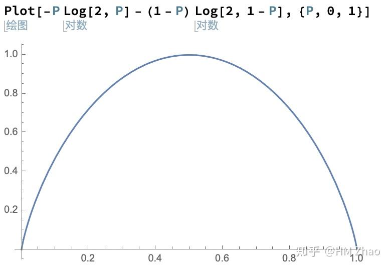
可以很容易看见，当系统状态完全确定，即 \(P=0,1\) 时，信息熵为零，而系统状态完全不确定，即 \(P=0.5\) 呈均匀分布时，信息熵取到最大值 \(1~\text{bit}\) 。因此，信息熵越小，表明我们对该系统了解越多，信息熵的下界也就代表了我们能了解的最多信息。

It is easy to see that when the state is completely certain, \(P=0,1\), the entropy is zero. When the state is completely uncertain, with the uniform distribution \(P=0.5\), the entropy reaches its maximum, \(1~\text{bit}\). So the smaller the entropy, the more we know about the system. A lower bound on entropy therefore represents the most information we can have.

方便起见，我们在接下来的计算中选取自然对数，信息熵的单位为nat。

For convenience, we will use natural logarithms in the calculations below, so entropy is measured in nats.

为了刻画不确定性关系，我们首先需要把信息熵推广至连续变量的情形，即用概率密度函数 \(p\to p(x)dx\) 代替概率：

To describe the uncertainty relation, we first need to extend information entropy to continuous variables, replacing probabilities with a probability density \(p\to p(x)dx\):

\[\begin{align*} H_x &= -\lim_{\Delta x\to 0}\sum_{\Delta x} p(x)\Delta x\log(p(x)\Delta x)\\ &=-\lim_{\Delta x\to 0}\sum_{\Delta x} p(x)\Delta x(\log p(x)+\log\Delta x)\\ &=-\lim_{\Delta x\to 0}\sum_{\Delta x} p(x)\log p(x)\Delta x-\lim_{\Delta x\to 0}\log\Delta x\sum_{\Delta x}p(x)\Delta x\\ &=-\int p(x)\log p(x) d x - \lim_{\Delta x\to 0}\log\Delta x\int p(x)d x, \end{align*}\\\]

\[\begin{align*} H_x &= -\lim_{\Delta x\to 0}\sum_{\Delta x} p(x)\Delta x\log(p(x)\Delta x)\\ &=-\lim_{\Delta x\to 0}\sum_{\Delta x} p(x)\Delta x(\log p(x)+\log\Delta x)\\ &=-\lim_{\Delta x\to 0}\sum_{\Delta x} p(x)\log p(x)\Delta x-\lim_{\Delta x\to 0}\log\Delta x\sum_{\Delta x}p(x)\Delta x\\ &=-\int p(x)\log p(x) d x - \lim_{\Delta x\to 0}\log\Delta x\int p(x)d x, \end{align*}\\\]

利用概率密度的归一化性 \(\int p(x)d x=1, \) 有
\[ \begin{align} H_x=-\int p(x)\log p(x) d x - \lim_{\Delta x\to 0}\log\Delta x. \end{align}\\\]

Using the normalization of the probability density, \(\int p(x)d x=1, \), we have
\[ \begin{align} H_x=-\int p(x)\log p(x) d x - \lim_{\Delta x\to 0}\log\Delta x. \end{align}\\\]

这里保留了 \(\Delta x\) ，目的是保护量纲。

I have kept \(\Delta x\) here to preserve the dimensions.

下面我们来考虑不确定性最小的情形，以已归一化的高斯波包（如谐振子基态）为例，波函数^[1]

Now consider the case of minimum uncertainty. Take a normalized Gaussian wave packet, such as the ground state of a harmonic oscillator. Its wavefunction is^[1]

\[\psi(x)= \frac{1}{(2\pi)^{1/4}\sqrt{\delta x}}e^{-\frac{x^2}{4(\delta x)^2}+\frac{i}{\hbar}p_0x},\\\]

\[\psi(x)= \frac{1}{(2\pi)^{1/4}\sqrt{\delta x}}e^{-\frac{x^2}{4(\delta x)^2}+\frac{i}{\hbar}p_0x},\\\]

其中引入了参数 \(\delta x, p_0\) ，容易发现它们分别对应于坐标的标准差和动量的平均值。

We have introduced the parameters \(\delta x, p_0\). It is easy to see that they correspond to the standard deviation of position and the mean momentum, respectively.

由波函数可得概率分布

The wavefunction gives the probability distribution

\[p(x) = |\psi(x, t)|^2 = \frac{1}{\sqrt{2\pi}\delta x}e^{-\frac{x^2}{2(\delta x)^2}},\\\]

\[p(x) = |\psi(x, t)|^2 = \frac{1}{\sqrt{2\pi}\delta x}e^{-\frac{x^2}{2(\delta x)^2}},\\\]

接着经过计算（塞进Mathematica）可得对应信息熵（后来查文献^[2]发现一般称为坐标熵position entropy）

A calculation—meaning, I put it into Mathematica—then gives the corresponding information entropy. I later found in the literature^[2] that this is usually called position entropy:

\[H_x=\log(\sqrt{2\pi}\delta x)+\frac{1}{2} - \lim_{\Delta x\to 0}\log\Delta x,\\\]

\[H_x=\log(\sqrt{2\pi}\delta x)+\frac{1}{2} - \lim_{\Delta x\to 0}\log\Delta x,\\\]

我们依然因为量纲的缘故保留了 \(\Delta x\) ，而一般文献^[2]将其视为常数而忽略。

Again, I have kept \(\Delta x\) for dimensional reasons, whereas the literature^[2] generally treats it as a constant and drops it.

为了计算动量对应的信息熵，我们接着考虑波包在动量表象下的分布，利用傅里叶变换得

To calculate the information entropy associated with momentum, we next consider the wave packet in the momentum representation. A Fourier transform gives

\[\begin{align} \tilde{\psi}(p_x) &= \frac{1}{\sqrt{2\pi\hbar}}\int_{-\infty}^\infty\psi(x)e^{-\frac{i}{\hbar}p_x x}d x\\ &=\left(\frac{2}{\pi}\right)^{1/4}\sqrt{\frac{\delta x}{\hbar}}e^{-\frac{(\delta x)^2(p_x-p_0)^2}{\hbar^2}}, \end{align}\\\]

\[\begin{align} \tilde{\psi}(p_x) &= \frac{1}{\sqrt{2\pi\hbar}}\int_{-\infty}^\infty\psi(x)e^{-\frac{i}{\hbar}p_x x}d x\\ &=\left(\frac{2}{\pi}\right)^{1/4}\sqrt{\frac{\delta x}{\hbar}}e^{-\frac{(\delta x)^2(p_x-p_0)^2}{\hbar^2}}, \end{align}\\\]

对应概率分布为

The corresponding probability distribution is

\[\begin{align} p(p_x) &=|\tilde{\psi}(p_x)|^2\\ &=\sqrt{\frac{2}{\pi}}\frac{\delta x}{\hbar}e^{\frac{(p_x-p_0)^2}{2(\hbar/{2\delta x})^2}}, \end{align}\\\]

\[\begin{align} p(p_x) &=|\tilde{\psi}(p_x)|^2\\ &=\sqrt{\frac{2}{\pi}}\frac{\delta x}{\hbar}e^{\frac{(p_x-p_0)^2}{2(\hbar/{2\delta x})^2}}, \end{align}\\\]

可见确实有 \(\begin{align*} \delta p_x=\frac{\hbar}{2\delta x}, \end{align*}\) 即不确定关系 \[\begin{align} \delta x\delta p_x=\frac{\hbar}{2}. \end{align}\\\]

We can see that \(\begin{align*} \delta p_x=\frac{\hbar}{2\delta x}, \end{align*}\) does indeed hold, giving the uncertainty relation \[\begin{align} \delta x\delta p_x=\frac{\hbar}{2}. \end{align}\\\].

同样计算可得其信息熵（称为动量熵momentum entropy）为

The same calculation gives its information entropy, called momentum entropy:

\[\begin{align} H_{p_x}= \log(\sqrt{\frac{\pi}{2}}\frac{\hbar}{\delta x})+\frac{1}{2} - \lim_{\Delta p_x\to 0}\log\Delta p_x. \end{align}\\\]

\[\begin{align} H_{p_x}= \log(\sqrt{\frac{\pi}{2}}\frac{\hbar}{\delta x})+\frac{1}{2} - \lim_{\Delta p_x\to 0}\log\Delta p_x. \end{align}\\\]

因此，这个高斯波包坐标与动量所蕴含的总信息熵为

Thus the total information entropy contained in the position and momentum of this Gaussian wave packet is

\[\begin{align*} H&=H_x+H_{p_x}\\&=\log(\pi\hbar)+1-\lim_{\Delta x, \Delta{p_x}\to 0}\log(\Delta x\Delta p_x)\\ &=\lim_{\Delta x, \Delta{p_x}\to 0}\log(\frac{h}{2\Delta x\Delta p_x})+1. \end{align*}\\\]

\[\begin{align*} H&=H_x+H_{p_x}\\&=\log(\pi\hbar)+1-\lim_{\Delta x, \Delta{p_x}\to 0}\log(\Delta x\Delta p_x)\\ &=\lim_{\Delta x, \Delta{p_x}\to 0}\log(\frac{h}{2\Delta x\Delta p_x})+1. \end{align*}\\\]

接下来需要处理 \(\Delta x,\Delta p\) ，如果他们真的趋于零的话，就会导致熵的发散，显然不行。但怎么取我也没有想得很明白，暂时使用的方案是量子统计里采用的取相空间最小体积为 \(h^3\) ，应用到此处就是取 \(\Delta x\Delta p_x\to h\) ，得到

We now have to deal with \(\Delta x,\Delta p\). If they really tend to zero, the entropy diverges, which clearly will not do. But I have not quite figured out how to choose them either. For now, I use the minimum phase-space volume \(h^3\) adopted in quantum statistics. Applied here, that means choosing \(\Delta x\Delta p_x\to h\), which gives

\[\begin{align} H=\log(\frac{1}{2})+1=\log(\frac{e}{2})=1-\frac{1}{\log_2{e}}, \end{align}\\\]

\[\begin{align} H=\log(\frac{1}{2})+1=\log(\frac{e}{2})=1-\frac{1}{\log_2{e}}, \end{align}\\\]

是一个与物理无关的纯常数！

A pure constant, with no physics in it!

加上单位，我们最终得到，不确定性关系所施加的信息熵限制为

Putting the units back in, we finally get the information-entropy bound imposed by the uncertainty relation:

\[\begin{align} \frac{H}{\text{nat}}\ge 1-\frac{1}{\log_2{e}}, \end{align}\\\]

\[\begin{align} \frac{H}{\text{nat}}\ge 1-\frac{1}{\log_2{e}}, \end{align}\\\]

比特形式为

In bits, this is

\[\begin{align} \frac{H}{\text{bit}}\ge \log_2{e}-1. \end{align}\\\]

\[\begin{align} \frac{H}{\text{bit}}\ge \log_2{e}-1. \end{align}\\\]

上述过程仅仅考虑了高斯波包的情形，一般情形据说可以使用Wigner Function证明。

The calculation above only considers a Gaussian wave packet. Apparently the general case can be proved using the Wigner function.

值得注意的是，由于这里考虑了\(\Delta x,\Delta p\) 的选取问题，并采用了统计力学中相空间体积元为 \(h^3\) 的方案，所以与许多文献中得到的结论 \(\log(\frac{he}{2})=\log(\pi\hbar)+1, \log\pi e\) 等有所不同，但究竟如何选取，我目前还没有很好的想法。

Note that I have considered how to choose \(\Delta x,\Delta p\) and adopted the statistical-mechanics prescription of a phase-space volume element \(h^3\). This differs from results such as \(\log(\frac{he}{2})=\log(\pi\hbar)+1, \log\pi e\) found in many papers. But I still do not have a good idea of what the right choice is.

另一个遗留问题是这里的熵的物理意义如何诠释。

Another unresolved question is how to interpret the physical meaning of this entropy.

理论上，以nat为单位的信息熵在乘上玻尔兹曼常数后，就是热力学熵（吉布斯熵）

In theory, information entropy in nats, multiplied by Boltzmann’s constant, gives thermodynamic entropy—the Gibbs entropy:

\[S=k_B\ln\Omega=-k_B\sum_i p_i\ln p_i,\\\]

\[S=k_B\ln\Omega=-k_B\sum_i p_i\ln p_i,\\\]

那么这里似乎可以得到一个单一波包由于量子效应具有一个最小的“熵”

So this seems to give a minimum “entropy” for a single wave packet arising from quantum effects:

\[S_0=k_B\ln\frac{e}{2},\\\]

\[S_0=k_B\ln\frac{e}{2},\\\]

而一个自由波包随着时间演化会扩散，即 \(\delta x\) 变大而 \(\delta p_x\) 不变，不再给出不确定关系的下界，而在这一过程中，上述定义的“熵”便会自发增加。

A free wave packet spreads as it evolves: \(\delta x\) grows while \(\delta p_x\) stays fixed, so it no longer saturates the uncertainty relation. In the process, the “entropy” defined above increases spontaneously.

如果考虑一个非自由的波包，如谐振子基态，由于它处于能量的本征态上，随着时间概率分布不会改变，似乎达到了某种“热平衡”。那么似乎就存在某种“温度”

For a wave packet that is not free, such as the ground state of a harmonic oscillator, the probability distribution does not change with time because it is an energy eigenstate. It seems to have reached some sort of “thermal equilibrium.” So there would seem to be some sort of “temperature”:

\[T_0=\frac{E_0}{S_0}=\frac{\frac{1}{2}\hbar\omega}{k_B\ln\frac{e}{2}}=\frac{\hbar\omega}{2k_B\ln\frac{e}{2}}.\\\]

\[T_0=\frac{E_0}{S_0}=\frac{\frac{1}{2}\hbar\omega}{k_B\ln\frac{e}{2}}=\frac{\hbar\omega}{2k_B\ln\frac{e}{2}}.\\\]

可是单个粒子何来熵与温度之说呢？同时这里出现的奇怪因子 \(\ln\frac{e}{2}\) 似乎从来没见过，这是否暗示我们一开始的选取方案错了？因为在经典情形下，谐振子热运动有两个自由度，由能均分定理应有 \(E=k_BT\) ，这要求没有因子 \(\ln\frac{e}{2}\) 。

But how can a single particle have entropy and temperature? And I do not recall ever seeing this strange factor \(\ln\frac{e}{2}\). Is that a hint that our choice at the outset was wrong? Classically, a harmonic oscillator has two degrees of freedom in thermal motion, so equipartition should give \(E=k_BT\). That requires the factor \(\ln\frac{e}{2}\) to be absent.

从另一方面说，如果采用李老师 @Triborg 在下文中的方法

On the other hand, if we use Professor Li’s (@Triborg) method from the following article,

谐振子相空间轨迹为椭圆，其体积为 \(Q=\int pdq=\pi \cdot m\omega A \cdot A=\frac{2\pi E}{\omega},\) 同样取相空间体积元大小为 \(h\) ，则微观状态数为 \(\Omega=\frac{Q}{h}=\frac{2\pi E}{h\omega}\) ，熵为 \(S=k_B\ln\Omega=k_B\ln\frac{E}{\hbar\omega}=k_B\ln\frac{1}{2}\) ，与前面所得正好相差了 \(1\) ，而反观前面的计算过程， \(\ln\frac{1}{2}\) 是由不确定性关系得到的，那个 \(1\) 却不是。可是文献^[2]中也得到了相同的 \(\ln\frac{e}{2}\) ，究竟问题出在哪呢？

the harmonic oscillator’s phase-space trajectory is an ellipse of volume \(Q=\int pdq=\pi \cdot m\omega A \cdot A=\frac{2\pi E}{\omega},\). Again taking the phase-space volume element to be \(h\) gives a number of microstates \(\Omega=\frac{Q}{h}=\frac{2\pi E}{h\omega}\) and entropy \(S=k_B\ln\Omega=k_B\ln\frac{E}{\hbar\omega}=k_B\ln\frac{1}{2}\). This differs from our earlier result by exactly \(1\). Looking back at the calculation, \(\ln\frac{1}{2}\) came from the uncertainty relation, but that \(1\) did not. Yet the literature^[2] gets the same \(\ln\frac{e}{2}\). Where exactly is the problem?

经李老师指点，上述论证的问题可能在于本质上还是经典统计：求谐振子相空间体积，然后除以相空间体积元大小，其实在计算的微观状态数是不同的 \((p, q)\) 组，而在量子情形下，波函数已经是对状态的完全描述了，而对于我们所考察的谐振子基态，微观状态数就是1，上述计算的熵就应当是0，可见上述过程计算的熵在量子语境下其实是冯诺依曼熵。

Professor Li pointed out that the problem with the argument above may be that it is still essentially classical statistics. Calculating the harmonic oscillator’s phase-space volume and dividing by the size of a phase-space cell really counts different \((p, q)\) pairs as microstates. In the quantum case, however, the wavefunction already gives a complete description of the state. For the oscillator ground state we are considering, there is just one microstate, and the entropy calculated that way should be zero. So in the quantum setting, the entropy computed by that procedure is actually the von Neumann entropy.

实际上一个谐振子更为主要的熵来源也应当是不同态叠加导致的冯诺依曼熵 \(S=-\text{tr}(\rho\ln\rho)\) ，但是我们为了将其剥离，仅考察不确定关系带来的熵，所以只讨论了谐振子基态，即在能量表象下态已完全确定，故不存在冯诺依曼熵。

In fact, the main source of entropy for an oscillator should also be the von Neumann entropy \(S=-\text{tr}(\rho\ln\rho)\) arising from a superposition of different states. But to separate this out and look only at the entropy coming from the uncertainty relation, we have considered only the oscillator ground state. Its state is completely specified in the energy representation, so there is no von Neumann entropy.

这里还有个问题就是，前面计算出的信息熵是一个和物理常量无关的常数，也就是说，取经典极限 \(\hbar\to 0\) 并不会使其消失！但这一熵的产生是完全基于量子机制的。因此，如果能将这一熵诠释为热力学熵的话，应当导致可观测的效应。

There is another puzzle here. The information entropy we calculated is a constant independent of physical constants. In other words, taking the classical limit \(\hbar\to 0\) does not make it disappear! Yet this entropy arises entirely from a quantum mechanism. So if it can be interpreted as thermodynamic entropy, it ought to have observable effects.

但一旦向经典极限走，谐振子就不会呆在基态了，因而会带来巨量的冯诺依曼熵淹没不确定性熵，最终回到经典统计的结果。

But as we move toward the classical limit, the oscillator no longer stays in its ground state. This brings in a huge amount of von Neumann entropy that overwhelms the uncertainty entropy, eventually recovering the classical-statistics result.

总而言之，这个计算结果的物理意义我目前还没太想明白，因此先把计算结果放这里。

Anyway, I still have not really figured out what this calculation means physically, so I will leave the result here for now.

检索的关键词真是非常重要，终于找到合适的关键词了：entropic uncertainty relation。

Search keywords really do matter. I finally found the right ones: entropic uncertainty relation.

看到wiki正中央框出来答案说明算对了还是蛮爽的:)

Seeing the answer boxed right in the middle of Wikipedia and realizing that I got it right feels pretty good :)

特别地，这一公式及相关量子力学量的信息量的诠释在Hugh Everett III提出多世界诠释的博士论文中首次提出并做了详细的阐述^[3]。

In particular, this formula and the interpretation of the information content of related quantum-mechanical quantities were first proposed and discussed in detail in Hugh Everett III’s doctoral dissertation introducing the many-worlds interpretation^[3].

不过这一公式的热力学解释我还没查到能看懂的，似乎还有很多近几年的相关文章（至少不是上个世纪的了）。

I still have not found a thermodynamic explanation of this formula that I can understand, though. There seem to be quite a few relevant papers from the last few years—at least they are not all from the last century anymore.

在这里计算的坐标熵和动量熵，在目前的literature中是operator entropy的特例，具体可见两篇PRE：

The position and momentum entropies calculated here are special cases of what the current literature calls operator entropy. See these two PRE papers:

Quantum operator entropies under unitary evolution

Quantum operator entropies under unitary evolution

Generalized Wigner–von Neumann entropy and its typicality

Generalized Wigner–von Neumann entropy and its typicality

这个做法最早可以追溯到von Neumann所证明的quantum H theorem：

This approach goes back to the quantum H-theorem proved by von Neumann:

Proof of the ergodic theorem and the H-theorem in quantum mechanics

Proof of the ergodic theorem and the H-theorem in quantum mechanics

1. ^朗道 量子力学
2. ^^abcLeipnik R. Entropy and the uncertainty principle[J]. Information and Control, 1959, 2(1): 64-79. https://www.sciencedirect.com/science/article/pii/S0019995859900828
3. ^ Hugh Everett, III. The Many-Worlds Interpretation of Quantum Mechanics: the theory of the universal wave function. Everett's Dissertation https://www.pbs.org/wgbh/nova/manyworlds/pdf/dissertation.pdf

1. ^Landau, Quantum Mechanics
2. ^^abcLeipnik R. Entropy and the uncertainty principle[J]. Information and Control, 1959, 2(1): 64-79. https://www.sciencedirect.com/science/article/pii/S0019995859900828
3. ^ Hugh Everett, III. The Many-Worlds Interpretation of Quantum Mechanics: the theory of the universal wave function. Everett's Dissertation https://www.pbs.org/wgbh/nova/manyworlds/pdf/dissertation.pdf