Using Conformal Transformation to Solve Electrostatic Problems

刚开始学习电磁学时就听说过保角变换法，可是直接看复变函数/电动力学中的保角变换部分过于困难，知乎上又少有对如何使用保角变换法解决静电场问题的介绍，因此我也一直没有机会了解这种高端的方法。这次质心冬令营讲解了一些相关内容，我便根据自己的理解，将保角变换法的相关内容记录于此文中。

I heard about conformal mapping when I first started learning electromagnetism. But jumping straight into the conformal-mapping sections of complex analysis or electrodynamics was too hard, and there was not much on Zhihu about actually using it to solve electrostatics problems. So I never really got a chance to learn this fancy technique. This time, the Zhixin physics Olympiad winter camp covered some of it, and I thought I would write down what I understood here.

解析/全纯函数是复变函数中的一个基本概念，它指的是复平面上处处可微的一类复变函数。

Analytic, or holomorphic, functions are a basic concept in complex analysis: complex functions that are differentiable everywhere on the complex plane.

解析函数需要满足柯西-黎曼条件。简单地说（无视严谨性），复平面上可微，就是说极限 \(\lim_{\Delta z \rightarrow 0} \frac{f(z+\Delta z)-f(z)}{\Delta z}\) 要存在，其中 \(z=x+iy, \ \ \ \ x, y \in \mathbb{R}\) ， \(f(z)=\phi(z)+i\psi(z), \ \ \ \phi(z),\psi(z)\in\mathbb{R}\) 。

An analytic function must satisfy the Cauchy–Riemann conditions. Roughly speaking, and never mind rigor for a moment, being differentiable on the complex plane means that the limit \(\lim_{\Delta z \rightarrow 0} \frac{f(z+\Delta z)-f(z)}{\Delta z}\) exists, where \(z=x+iy, \ \ \ \ x, y \in \mathbb{R}\) and \(f(z)=\phi(z)+i\psi(z), \ \ \ \phi(z),\psi(z)\in\mathbb{R}\).

把 \(z\) 和 \(f\) 代入，将分子凑出因子 \(\Delta x+i\Delta y\) 之后，即可得到柯西-黎曼条件： \(\frac{\partial \phi}{\partial x}=\frac{\partial \psi}{\partial y}, \frac{\partial \phi}{\partial y}=-\frac{\partial \psi}{\partial x}\) 。

Substitute \(z\) and \(f\) and rearrange the numerator to factor out \(\Delta x+i\Delta y\). This gives the Cauchy–Riemann conditions: \(\frac{\partial \phi}{\partial x}=\frac{\partial \psi}{\partial y}, \frac{\partial \phi}{\partial y}=-\frac{\partial \psi}{\partial x}\).

这个条件很有意思，他实际上说明了 \(\phi, \psi\) 都满足拉普拉斯方程，以 \(\phi\) 为例： \(\nabla^2 \phi = \frac{\partial^2 \phi}{\partial x^2}+\frac{\partial^2 \phi}{\partial y^2} = \frac{\partial}{\partial x}\frac{\partial \phi}{\partial x}+\frac{\partial}{\partial y}\frac{\partial \phi}{\partial y}=\frac{\partial}{\partial x}\frac{\partial \psi}{\partial y}-\frac{\partial}{\partial y}\frac{\partial \psi}{\partial x}=0\) 。

This is an interesting condition: it actually tells us that \(\phi, \psi\) both satisfy Laplace’s equation. Taking \(\phi\) as an example: \(\nabla^2 \phi = \frac{\partial^2 \phi}{\partial x^2}+\frac{\partial^2 \phi}{\partial y^2} = \frac{\partial}{\partial x}\frac{\partial \phi}{\partial x}+\frac{\partial}{\partial y}\frac{\partial \phi}{\partial y}=\frac{\partial}{\partial x}\frac{\partial \psi}{\partial y}-\frac{\partial}{\partial y}\frac{\partial \psi}{\partial x}=0\).

因此，我们便可以将电势作为其中的一个，比如 \(\phi(z)\) 。

We can therefore take the electric potential to be one of them, say \(\phi(z)\).

找一个性质比较好的映射 \(z^\prime: \mathbb{C} \rightarrow\mathbb{C}\) ，把原复平面上的点 \(z\) 映射至一个新的点 \(z^\prime(z)\) 。

Find a reasonably well-behaved mapping \(z^\prime: \mathbb{C} \rightarrow\mathbb{C}\) that takes a point \(z\) in the original complex plane to a new point \(z^\prime(z)\).

此时原复平面上的边界及电势 \(\Sigma_i, \phi(z)\) 也会映射到新的边界和电势 \(\Sigma^\prime_i, \phi^\prime(z^\prime)\) 。

The boundary and potential \(\Sigma_i, \phi(z)\) in the original complex plane are then mapped to a new boundary and potential \(\Sigma^\prime_i, \phi^\prime(z^\prime)\).

如果我们使新的边界条件与原边界条件相同，由于电势均满足拉普拉斯方程，于是就会有 \(\phi(z)=\phi^\prime(z^\prime)\) 。

If we impose the same boundary conditions in the new plane as in the original one, then, since both potentials satisfy Laplace’s equation, we have \(\phi(z)=\phi^\prime(z^\prime)\).

若选取合适的映射 \(z^\prime\) ，将原来复杂的边界映射到简单边界，在新复平面中解出电势 \(\phi^\prime\) ，再回到原复平面中，即可得到原来待求解的电势 \(\phi\) 。

Choose a suitable mapping \(z^\prime\) to turn a complicated boundary into a simple one, solve for the potential \(\phi^\prime\) in the new complex plane, and then map back to the original plane. This gives the potential we wanted, \(\phi\).

这就是保角变换解决平面静电学问题的基本思路。

That is the basic idea behind using conformal mapping to solve two-dimensional electrostatics problems.

值得注意的是，对于一般的三维问题，只要其具有某一方向上的平移对称性，即可转化为平面问题。

One thing to note: a general three-dimensional problem can be reduced to a two-dimensional problem as long as it has translational symmetry in some direction.

用 \(A=\frac{\text{d}z^\prime}{\text{d}z}\) 刻画变换前后长度的变化，

Use \(A=\frac{\text{d}z^\prime}{\text{d}z}\) to describe how lengths change under the transformation.

则变换前后的电场满足 \(E^\prime=-\frac{\text{d}\phi^\prime}{\text{d}z^\prime}=-\frac{\text{d}\phi}{\text{d}z}/\frac{\text{d}z^\prime}{\text{d}z}=E/\frac{\text{d}z^\prime}{\text{d}z}=E/A\) 。

The electric fields before and after the transformation then satisfy \(E^\prime=-\frac{\text{d}\phi^\prime}{\text{d}z^\prime}=-\frac{\text{d}\phi}{\text{d}z}/\frac{\text{d}z^\prime}{\text{d}z}=E/\frac{\text{d}z^\prime}{\text{d}z}=E/A\).

电荷量不变，线电荷密度由于线方向垂直于纸面，故不发生改变，面电荷密度则有 \(\sigma^\prime=\sigma/A\) 。

Charge is unchanged. The line charge density is also unchanged, because the line runs perpendicular to the page. The surface charge density, on the other hand, satisfies \(\sigma^\prime=\sigma/A\).

电容 \(C=\frac{Q}{\Delta\phi}\) 不变。

The capacitance \(C=\frac{Q}{\Delta\phi}\) is unchanged.

我们可以先从一些常见的函数入手：

We can start with a few familiar functions:

幂函数 \(z^\prime=z^n\)

Power functions \(z^\prime=z^n\)

复数 \(z=re^{i\theta}\) ，经过变换得到 \(z^\prime=r^ne^{in\theta}\) 。

The complex number \(z=re^{i\theta}\) becomes \(z^\prime=r^ne^{in\theta}\) under this transformation.

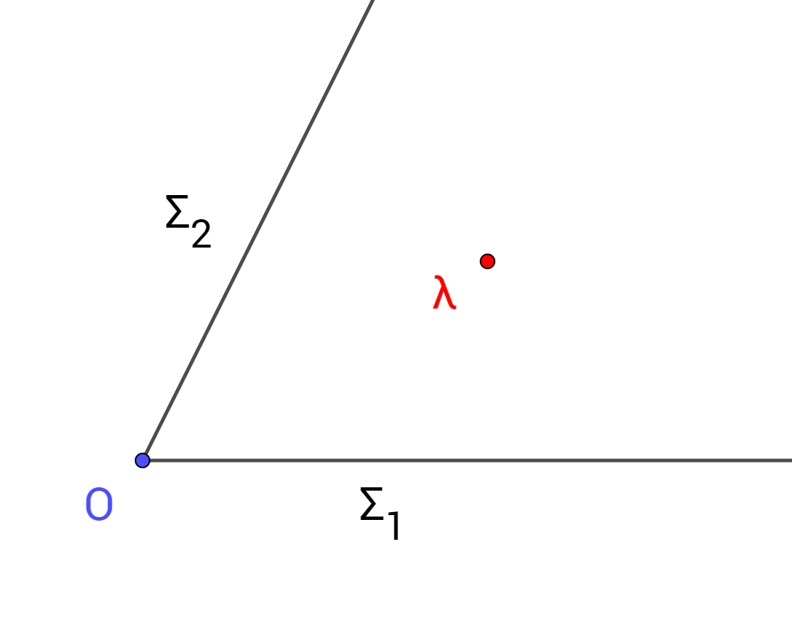
考察这样的一类边界：

Consider a boundary like this:

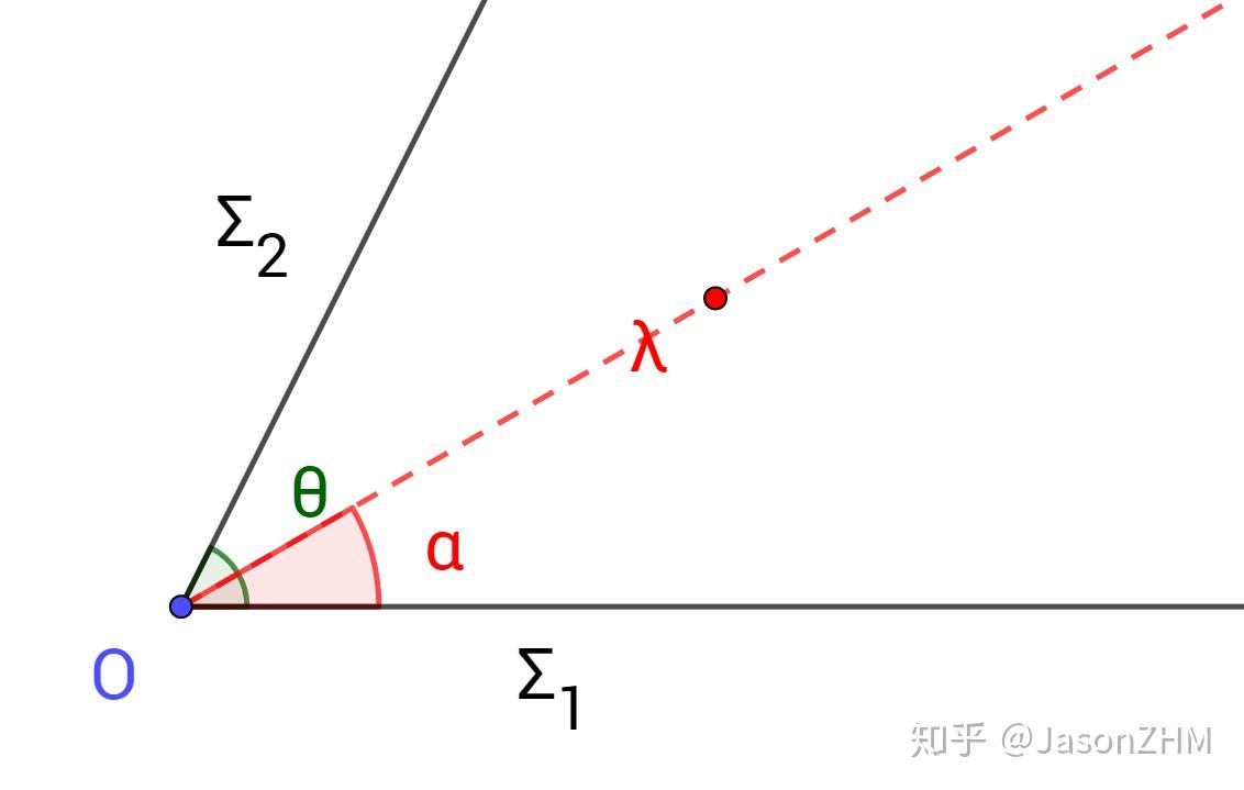
经过变换后， \(\Sigma_1\) 仅伸缩不旋转， \(\Sigma_2\) 伸缩后辐角变为 \(n\theta\) 。

Under the transformation, \(\Sigma_1\) is stretched but not rotated, while \(\Sigma_2\) is stretched and its argument becomes \(n\theta\).

如果我们选取 \(n=\frac{\pi}{\theta}\) ，那么角就会被拉平。

If we choose \(n=\frac{\pi}{\theta}\), the corner is flattened out.

如果原平面 \(\alpha\) 角处有一线电荷密度为 \(\lambda\) 的均匀带电长直导线，我们想要求解电势、电场分布以及导线受力，原本需要暴算无限发散电像法，现在就可以应用保角变换 \(z^\prime=z^{\pi/\theta}\) ，使得问题转化为：

Suppose a long, straight, uniformly charged wire with line charge density \(\lambda\) lies at the angle \(\alpha\) in the original plane, and we want the potential, electric-field distribution, and force on the wire. Originally, this would call for a brute-force, endlessly proliferating construction of image charges. Now we can apply the conformal mapping \(z^\prime=z^{\pi/\theta}\) and turn the problem into this:

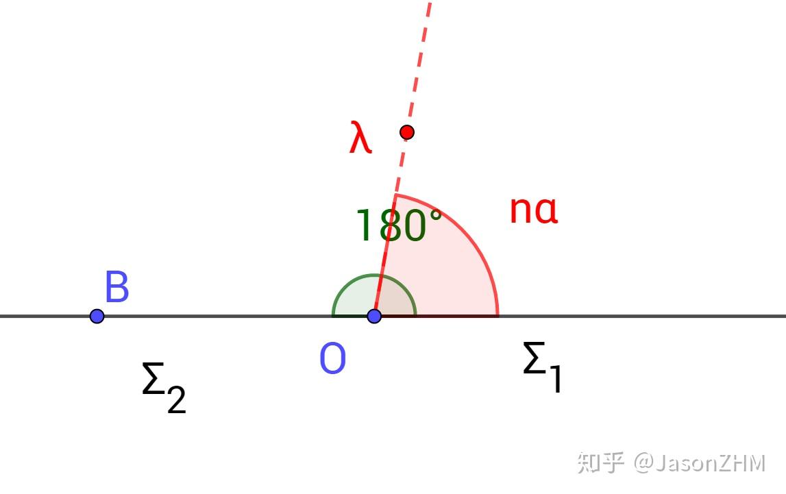
接下来只需要在平面下方作出对称的一个电像即可解得 \(\phi^\prime, E^\prime\) ，于是就得到 \(\phi=\phi^\prime, E=AE^\prime\) ，问题解决。

All that remains is to place a single symmetric image charge below the plane to find \(\phi^\prime, E^\prime\). We then have \(\phi=\phi^\prime, E=AE^\prime\). Problem solved.

对数函数 \(z^\prime=\ln z\)

Logarithmic functions \(z^\prime=\ln z\)

复数 \(z=re^{i\theta}\) ，经过变换得到 \(z^\prime=\ln{r} +i\theta\) ，即横坐标变为 \(\ln r\) ，纵坐标变为 \(\theta\) 。

The complex number \(z=re^{i\theta}\) becomes \(z^\prime=\ln{r} +i\theta\): the horizontal coordinate becomes \(\ln r\) and the vertical coordinate \(\theta\).

考察这样的一类边界，我们想要求解其电容：

Consider the following boundary. We want to find its capacitance:

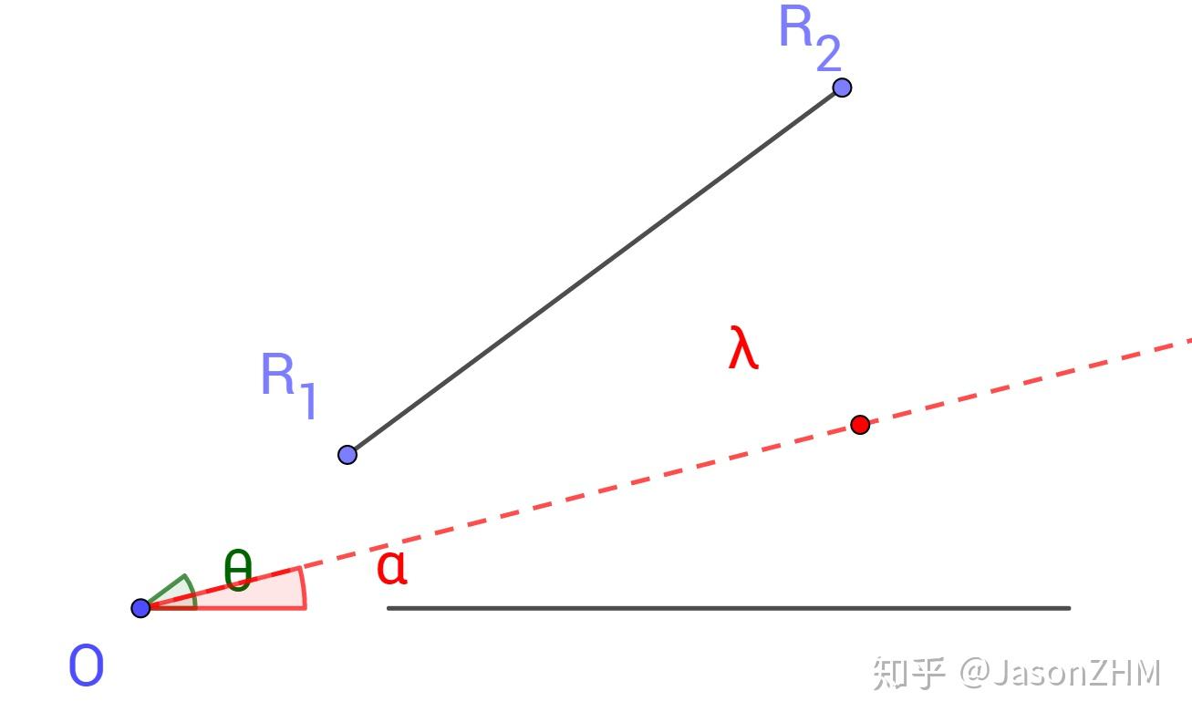
经过变换后，变为间距 \(\theta\) ，板宽 \(\ln{{R_2}}-\ln{{R_1}}\) 的两平行极板，问题一下子就简单了很多，解决后再变换回来即可。

The transformation turns it into two parallel plates separated by \(\theta\), with plate width \(\ln{{R_2}}-\ln{{R_1}}\). Suddenly the problem is much simpler. Solve it, then transform back.

指数函数 \(z^\prime=e^z\) 则恰恰相反，把带状区域映射为角型区域。

The exponential function \(z^\prime=e^z\) does exactly the reverse: it maps a strip into a wedge.

反演映射 \(z^\prime=\frac{1}{z}\)

Inversion \(z^\prime=\frac{1}{z}\)

考察复平面上的一个圆及其内部 \(\rho\leq2r \cos\theta\) ，经过变换得到 \(z^\prime=\frac{1}{\rho e^{i\theta}}=\frac{1}{2r}\frac{e^{-i\theta}}{\cos(-\theta)}=\rho^\prime e^{i\theta^\prime}\) ，于是 \(\theta^\prime=-\theta,\ \ \ \rho^\prime cos\theta^\prime =x^\prime\geq \frac{1}{2r}\) ，即直线 \(x^\prime=\frac{1}{2r}\) 及其右侧。

Consider a circle and its interior in the complex plane, \(\rho\leq2r \cos\theta\). The transformation gives \(z^\prime=\frac{1}{\rho e^{i\theta}}=\frac{1}{2r}\frac{e^{-i\theta}}{\cos(-\theta)}=\rho^\prime e^{i\theta^\prime}\), and hence \(\theta^\prime=-\theta,\ \ \ \rho^\prime cos\theta^\prime =x^\prime\geq \frac{1}{2r}\): the straight line \(x^\prime=\frac{1}{2r}\) and the region to its right.

该变换可以将圆边界变换为直线边界。

This transformation turns a circular boundary into a straight one.

读者可以通过借此证明球面电像法小试牛刀。

Try your hand at using this to prove the image-charge construction for a sphere.

反演变换的推广是分式型变换 \(z^\prime=\frac{az+b}{cz+d}\) 。

A generalization of inversion is the linear fractional transformation \(z^\prime=\frac{az+b}{cz+d}\).

三角函数 \(z^\prime=\sin z\)

Trigonometric functions \(z^\prime=\sin z\)

变换后 \(z^\prime=\sin(x+iy)=\sin x\cos iy+\cos x\sin iy=\sin x\cosh y+i\cos x\sinh y=x^\prime+iy^\prime\) ，所以有 \(x^\prime=\sin x\cosh y, ~y^\prime=\cos x\sinh y\)，此为双曲坐标系的标准形式 。

After the transformation, \(z^\prime=\sin(x+iy)=\sin x\cos iy+\cos x\sin iy=\sin x\cosh y+i\cos x\sinh y=x^\prime+iy^\prime\), so \(x^\prime=\sin x\cosh y, ~y^\prime=\cos x\sinh y\), the standard form of hyperbolic coordinates.

故当 \(y=const.\) ，即原边界为一水平直线时，新边界为一椭圆；

Thus, when \(y=const.\)—when the original boundary is a horizontal line—the new boundary is an ellipse;

当 \(x=const.\) 时，新边界为双曲线。

when \(x=const.\), the new boundary is a hyperbola.

因此，可以用(反)三角函数实现直线、椭圆、双曲线之间的互换。

So trigonometric functions and their inverses let us transform between straight lines, ellipses, and hyperbolas.

复合

Composition

通过上述几种基本的保角变换，可以通过连续的多次变换处理更为复杂的边界。

By applying these basic conformal mappings in succession, we can handle more complicated boundaries.

如果有什么边界是一次保角变换简化不了的，那就做两次。

If there is a boundary you cannot simplify with one conformal mapping, do two.